

Apache Spark is an open-source, distributed processing system used for big data workloads. It utilises in-memory caching, and optimised query execution for fast analytic queries against data of any size. It provides development APIs in Java, Scala, Python and R, and supports code reuse across multiple workloads—batch processing, interactive queries, real-time analytics, machine learning, and graph processing.
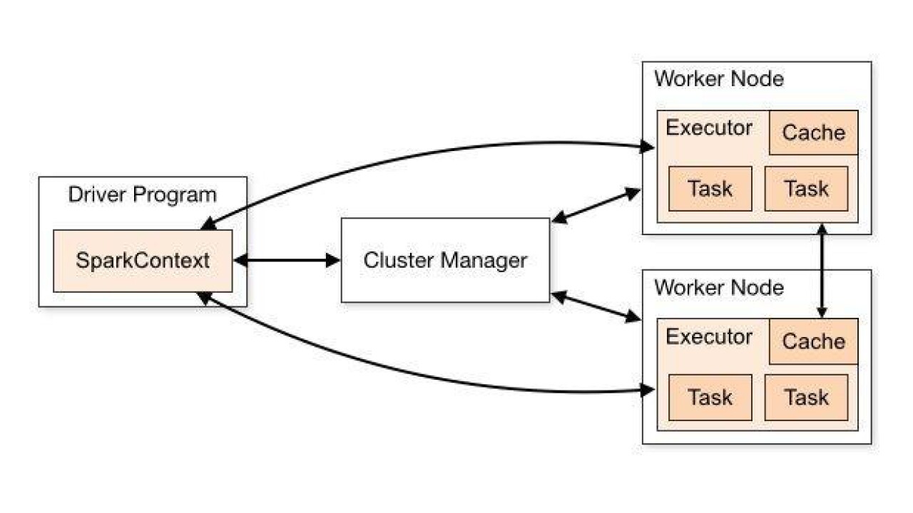 Visual Representation of Spark Architecture
 A Spark application consists of a driver process and a set of executor processes. The driver is a Java process where the main method of a spark application runs. It is responsible for creating multiple tasks and scheduling them to run on the executors. The executors are where the actual computation happens after the driver assigns tasks for them. An executor has majorly two responsibilities, executing code assigned to it by the driver and reporting the state of the computation back to the driver node. An executer having “n” cores can perform a maximum of “n” tasks at a time.
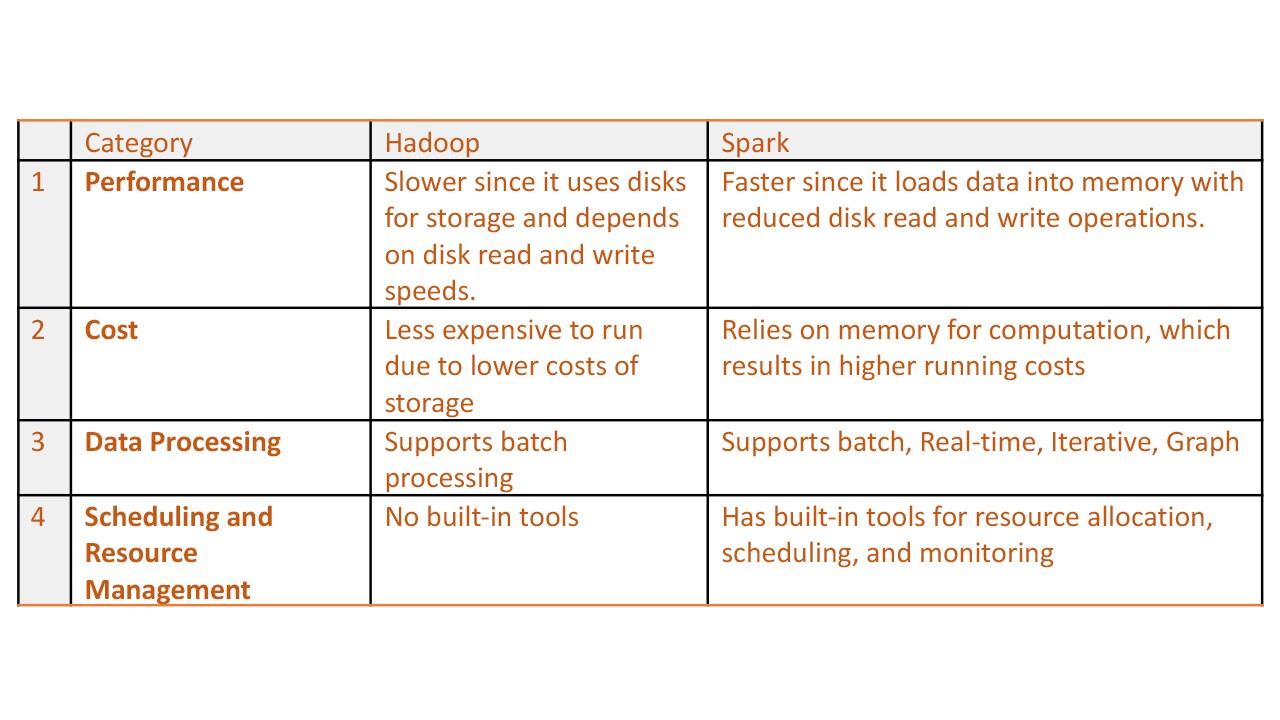 Spark: Comparison with Hadoop
Techniques to maximise the resource utilisation
Ideal Partitioning
While working on spark, one has to deal with executor configurations and data partitioning to get the optimal output in terms of resource utilisation. Partitioning is division of data into chunks. When an action is to be performed on a partitioned data, spark creates a job and transforms it into a Directed Acyclic Graph (DAG) based execution plan where each node within a DAG creates multiple stages. The number of partitions decide how many tasks are to be generated per stage.
While working on spark, one has to deal with executor configurations and data partitioning to get the optimal output in terms of resource utilisation. Partitioning is division of data into chunks. When an action is to be performed on a partitioned data, spark creates a job and transforms it into a Directed Acyclic Graph (DAG) based execution plan where each node within a DAG creates multiple stages. The number of partitions decide how many tasks are to be generated per stage.
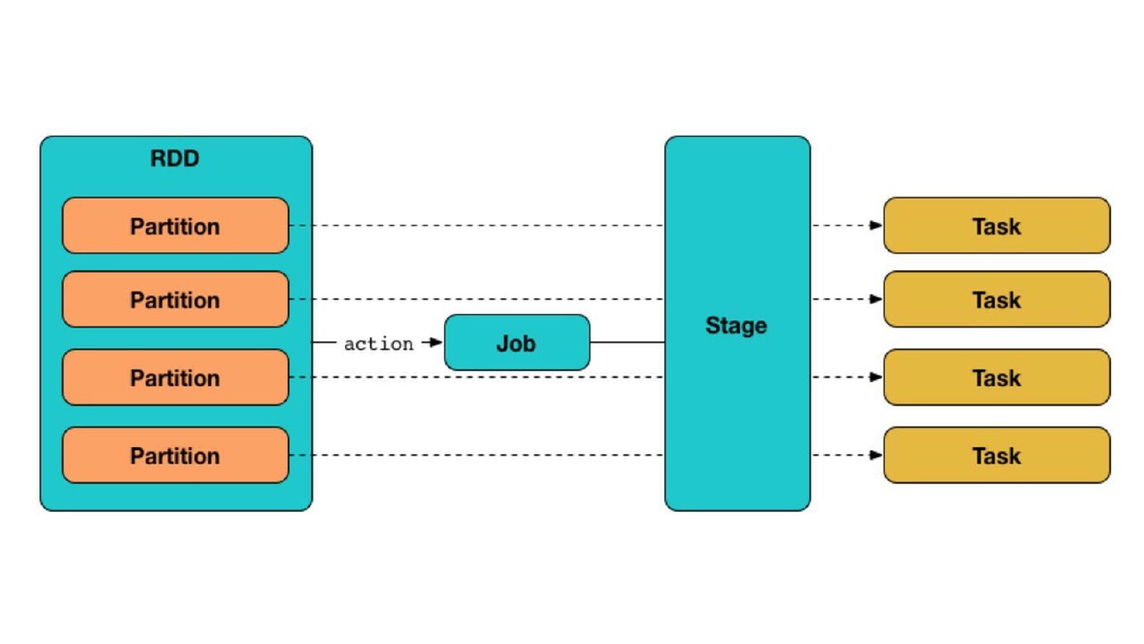 Visual representation of how a partition is mapped to a task
The intent behind data partitioning is to optimise the spark job's performance. The job runtime can be reduced by carefully distributing the input dataset into smaller chunks and processing these via Spark executors. Since there is no single thumb rule on how to partition your data in the best way, one's understanding of Spark internals and familiarity with the dataset becomes a crucial factor. Here are some of the common points to consider while partitioning the data:
a. Exorbitant number of partitions will result in too many tasks being created and will incur a scheduling overhead.
b. Low number of partitions will result in a smaller number of tasks being created. The lesser the number of tasks, lower will be the parallelisation making the job runtime longer than expected. The size of a single partition will also be high which could lead to ingesting high volume of data into a core resulting in OOM issues.
c. Skewed data in the partitions can result in unequal partitions in terms of data volume due to which some of the tasks might run relatively longer than the others.
If you know distribution of the data already, one can repartition over the uniformly distributed column in the dataframe.
df.repartition(<n_partitions>, <col_name>)
df.repartition(<n_partitions>, <col_name>)
The other way could be to add a salt column with random values and then partition over it. The randomness ensures no skewness over partitions.
import pyspark.sql.functions as F
df = df.withColumn('salt', F.rand())
df = df.repartition(, 'salt')
df = df.withColumn('salt', F.rand())
df = df.repartition(, 'salt')
This article will walk you through on how we partitioned the dataset to optimise the performance of the spark job in our production system where a workflow used to take more than the expected time to complete. One of the workflow nodes with data input size of ~300GB resulted in the job taking ~3 hours to complete. The cluster configuration on which the execution took place was: 10 nodes with 16 cores, having 64GB RAM per node. As a part of root cause analysis, it was noticed that the resource utilisation was less than 20% for the job. The underlying reason was the executors were not configured to optimise for the computation in context.
The first optimisation that we made was to balance the workload on the executors. Each executor was configured to have 5 cores to achieve the objective with 150 cores available for computation (1 core per each node is leveraged for application overhead). With the mentioned configuration, the total of number executors to work with came out to be 30. Each node was then assigned 3 executors to work with an intention to distribute the burden uniformly. The available memory for each executor came out to be ~18GB. Here’s how the calculation was done:
Number of cores available = 150
Number of available executors = total cores/cores per executor = 150/5 = 30 Number of executors per node = total executors/ total nodes = 30/10 = 3
Memory size per executor = memory per node/executors per node = 64/3 = 21 GB. ~18GB after removing heap overhead which is ~10%
This exercise of distributing the work to each configured executor with the following configuration resulted in 4 times the resource utilisation and reduced the job time to ~50 minutes.
--executor-memory 18G —executor-cores 5 —num-executors=30
Once the executors were configured, we were further able to reduce the job time by ~10 minutes by partitioning the data basis the size. Since each executor as per the above configuration can take up 5 tasks in parallel, we partitioned the data into 30*5 partitions over a uniformly distributed column. This made sure that none of the cores were sitting idle and we had ample number of tasks to be computed at a given time.
Shuffle Reduction
Shuffling is the process of redistributing data between partitions. When you are dealing with multiple datasets, joining them is one of the common actions that a Spark application has to do. It generally requires shuffling which increases the execution time due to data movement between the worker nodes.
In our data pipeline, one of the input tables containing primary keys was relatively smaller in size (~3GB) but required a join with a much larger table (~200GB). This created a performance bottleneck as for such a small-sized table lots of unnecessary shuffling was taking place. This added to the job runtime. We ended up broadcasting the table to each worker node, completely avoided shuffling and reduce the execution time by ~5minutes.
This was achieved by using the broadcast method which is supported for the table sizes less than 8GB.
larger_df.join(broadcast(smaller_df), on=[‘key’], how=’inner’)
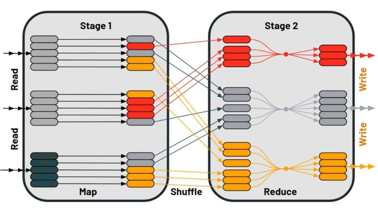 Visual representation of how rows are repartitioned between two stages using shuffling.
Optimising Reads
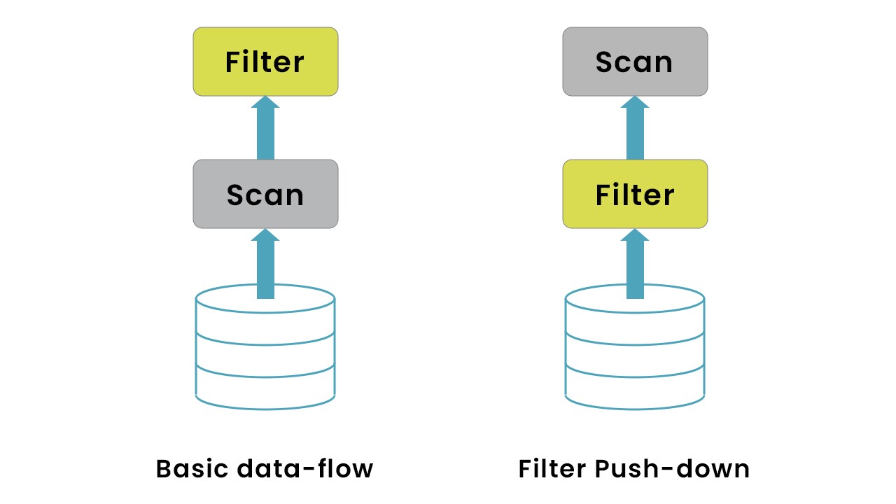
Reading is a crucial part of a spark application and is strongly coupled with how you are storing the data which is to be read. It is recommended to use columnar storage (Apache Parquet or Cassandra) to get the best read performance with Spark. When a read with select operation is executed, select col_1 from table1; Apache Parquet is designed to prevent the full data scan and selects only the queried columns. This reduces the load time unlike the traditional row-based datasets (CSV/TSV) which forces the spark application to scan the entire data before filtering. Parquet also supports compression of data. If your storage service is not free it significantly brings down the cost to store.
In our use case, the input data was of 1.2 TB and it required only a subset of data (query for the last 3 months) which was approximately ~300GB. Instead of loading the entire data snapshot into the Spark memory and then filtering out we restructured the input data and partitioned it basis the date - yyyy/mm/dd. On top of that, we were able to use the filter push-down capability of Parquet, loading only the required columns into the Spark memory. This resulted in ~25% performance and cost optimisation.
Caching Strategy
There are scenarios where a dataframe has to be re-used over and over again in the spark application. Caching in such scenarios would avoid the repetition of transformation loads. It is ideal to cache the dataframe post applying the required filters on it during the first few steps of a spark application. This can be simply done using cache() operation. Having a cache for every dataframe in greed of optimisation will be a misusage unless the spark application is running with an infinite memory pool. For better memory utilisation, one can unpersist() dataframe when your application no longer needs it.
Conclusions
- Spark partitioning minimises the shuffling. Hence, partitioning turns out very beneficial at the time of processing to reduce job runtime.
- Caching is an important technique to optimise spark jobs. We should cache our data if we are going to use it multiple times in our code. It can give us a significant performance benefit.
- Try to use Broadcast joins wherever possible and filter out the irrelevant rows to the join key to avoid unnecessary data shuffling.
- Prefer the compressed columnar data over CSVs/TSVs.
- Partition and store the input data on columns with high cardinality for faster retrieval.