Looking for AI-powered music recommendation tools? Amazon Sagemaker can help

Personalisation and recommender systems are at the core of almost every consumer application today. Modern digital consumerism has evolved pivoting heavily on personalisation, since introduced decades ago by Amazon e-commerce At the core of Indian classical music is its Ragas, which is a framework of a fixed set of notes and their movements as defined through its composition. With the provision for a musician to apply subtle improvisations on top of its theoretical note patterns, a Raga does portray distinct musical flavors, mood and ambience.

Indian music has diversified into numerous formats, originating from the ancient folk and classical genres. Despite this massive evolution, traces of Indian Ragas are still evident even in the most contemporary styles of Indian music. Application of Ragas still does help aesthetically portray an emotion in a song or situation. A well trained ear of a classical musician can easily detect such traces of Ragas in modern music.

The effectiveness of music recommendations based on their acoustic similarity is well established through several research works conducted in the last decade. A curiosity question can be - how is acoustic similarity determined ? It is determined with the help of multiple audio features such as melody, rhythm, genre, tempo, timbre, pitch descriptor, and several other low-level features. The audio feature list indicated above contributes to what our human ears perceive as acoustic similarity. This blog has two primary goals. First, it establishes how to determine acoustic similarities with the help of Raga based melody using machine learning. Secondly, it explains how managed machine learning services such as Amazon SageMaker can be leveraged to feature-engineer, train, optimize, and deploy complex deep learning models that are required for such use cases. Music businesses delivering direct-to-consumer music streaming experience will find actionable insights from this blog.

This blog will explore how to determine acoustic similarities with the help of Raga based melody.

Note: Readers are encouraged to familiarize themselves with core underlying topics such as Digital Signal Processing and Music Information Retrieval . This will help them to improvise and handle complex use cases around acoustic similarity in music.

It is imperative to numerically express the audio features referred to in the previous section. The audio features needed for this blog’s use case are amplitude, frequency, and mel-frequency-cepstral-coefficient (MFCC). We leverage open-source library Librosa for audio feature extraction. Librosa is distributed under ISC license and is a popular choice among developers working in the audio domain. Alternative libraries such as Essentia, audioFlux may also be reviewed for specific use cases.

Mel-Frequency-Cepstral-Coeffient (MFCC) is used as key input to the classifier model. MFCC is a set of coefficients that represent the audio spectral envelope. The spectral envelope is a representation of how the sound energy is distributed across different frequency bands. MFCCs are used in music classification because they capture the spectral characteristics of a sound that are most relevant for human perception of music. Below is a summary of standard steps for extraction of MFCC from an audio file,using Librosa.

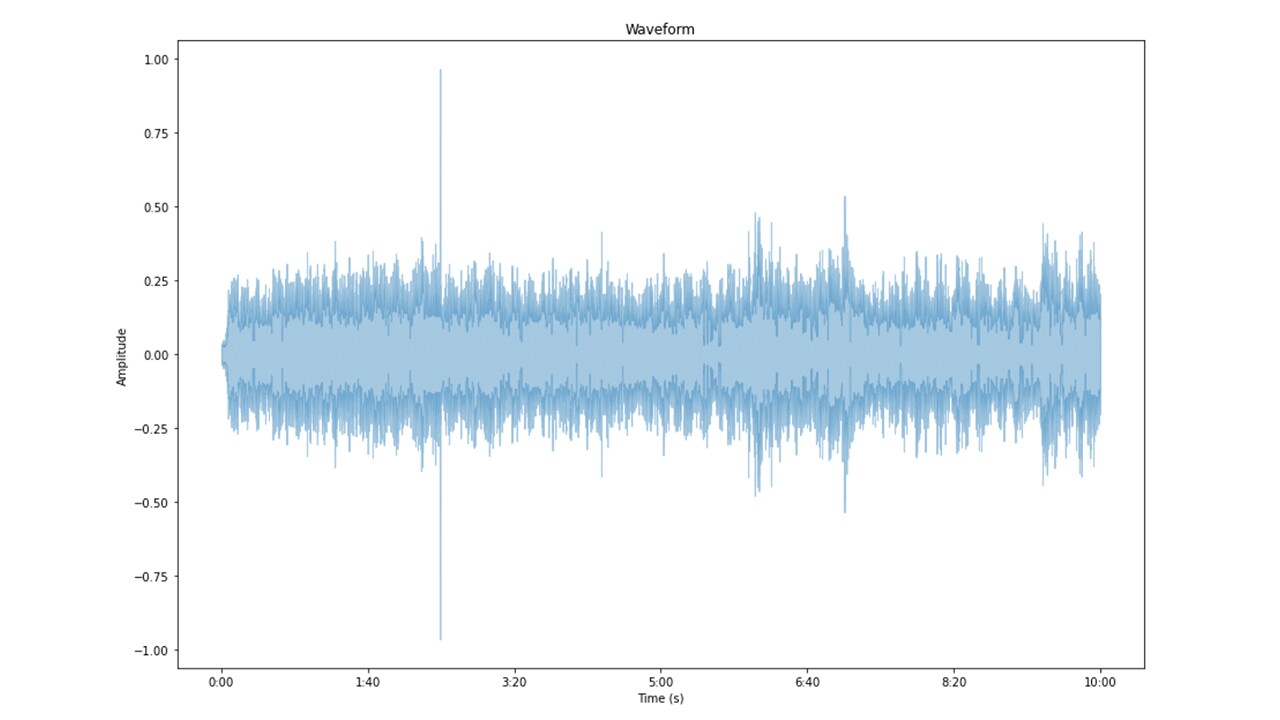
STEP 1 : Amplitude Determination – An audio file is loaded into the memory using Librosa, with a specified audio sampling rate. The API returns an audio signal object as a Python NumPy array. Each of the values of this NumPy array represents the amplitude of the audio waveform. The diagram below represents the amplitude in the time domain.

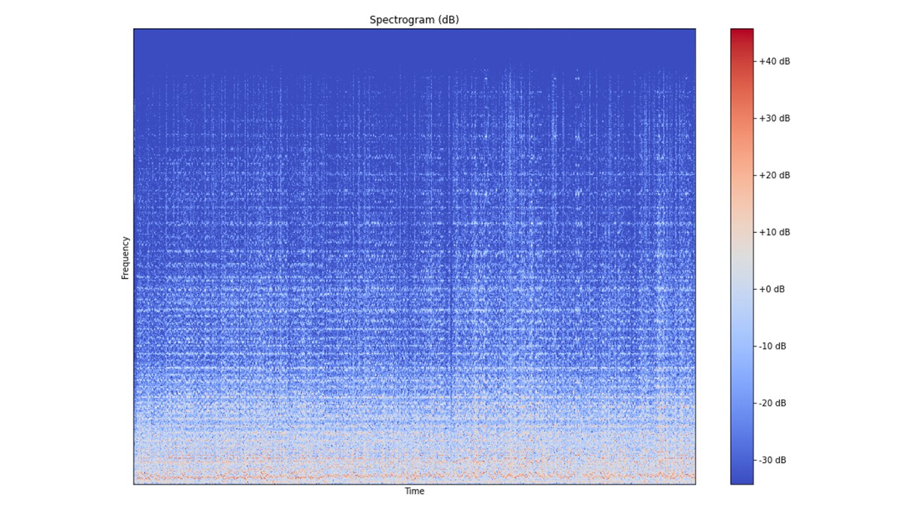
STEP 2 : Frequency Domain Transformation – To determine the frequency distribution of audio over a period of time, short-time-fourier-transform (STFT) is applied to generate a spectrogram plot. Spectrogram generation requires multiple inputs. First, it needs the number of samples per fast-fourier-transform (FFT). Expressed as an integer it indicates the number of samples for each of the FFT within the overall STFT. Secondly, spectrogram needs an input of the hop length. Expressed as an integer it indicates the magnitude of shift with each iteration of FFT. Overall, the spectrogram represents the audio amplitude value as a function of time and frequency. In order to articulate the spectrogram better, the amplitude distribution is converted into a logarithmic scale. The diagram below illustrates an audio frequency spectrogram in a logarithmic scale.

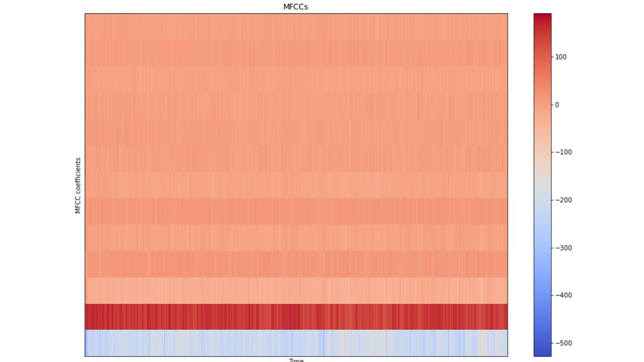
STEP 3 : Extract Mel-Frequency-Cepstral-Coefficient (MFCC) – MFCCs are computed using the Librosa API with an input comprising of the audio signal, number of samples per FFT, the hop length, and the number of MFCCs that needs to be extracted. The number of MFCC is typically set to 13 for music analysis. The diagram below illustrates a MFCC plot.

The objective of this blog is to build a classifier to identify traces of Indian Ragas in a song. Such a classifier would need labelled training data to be fed into a supervised machine learning model. Audio data is represented through multi-dimensional, complex, unstructured formats that would need deep neural network classifiers. This would also need a significant volume of training data balanced across different data classes. The section below summarizes the steps for training data preparation.

STEP 1 - RECORD TRAIN DATA : A set of Indian classical Ragas that are popularly found in modern songs was shortlisted. This included Ragas such as Yaman, Bhairavi, Khamaj, Kafi, etc. Each such Raga was played for approximately ten minutes on an Indian harmonium on C Sharp scale (C#). The Ragas were played impromptu without any planned notation. This was intentional, allowing the musician to improvise while playing, a situation representative of real-world Indian classical music demonstration. A careful iteration was done through the popular and mandatory notes and phrases of each Raga, to bring out the distinct musical flavors and emotions. Here is a link to a sample clip of Raga Yaman for reference.

STEP 2 - FEATURE GENERATION : Each of the ten minute pieces for individual Ragas (labeled data for training), was split into a collection of five second audio segments. While an even smaller sized segment of 1-2 seconds would have helped in augmenting the data volume and theoretically lowered the risk of over-fitting, there is a trade-off. A mere one second clip will fail to capture Raga specific information or frequency distribution. This would have lead to over-generalization and increased number of false positives during classification. The segment size was set to at least five seconds, such that at least one unique combination of the Raga phrases can be captured on the associated spectrogram. For each such five second segment, the MFCC value was computed (as explained in the previous section) and mapped to the label (The label is the name of the Raga). The final data structure looked as following:

data = [{“labels”: [], “mfcc”: []}, {“labels”: [], “mfcc”: []]

STEP 3 - RECORD TEST DATA SET: The previous two steps of creating music data, splitting into five second clips, and generating MFCC for each such clip was repeated again in this step, but for a set of popular film songs. This was to produce unseen test data to be used after training the model and to verify the accuracy of classification. For example, here a tune to a popular Hindi film song based on Raga Yaman. This data was used to test if the trained machine learning model was able to classify the underlying Raga of this song, with an acceptable level of accuracy. These audio samples were not used for the model training.

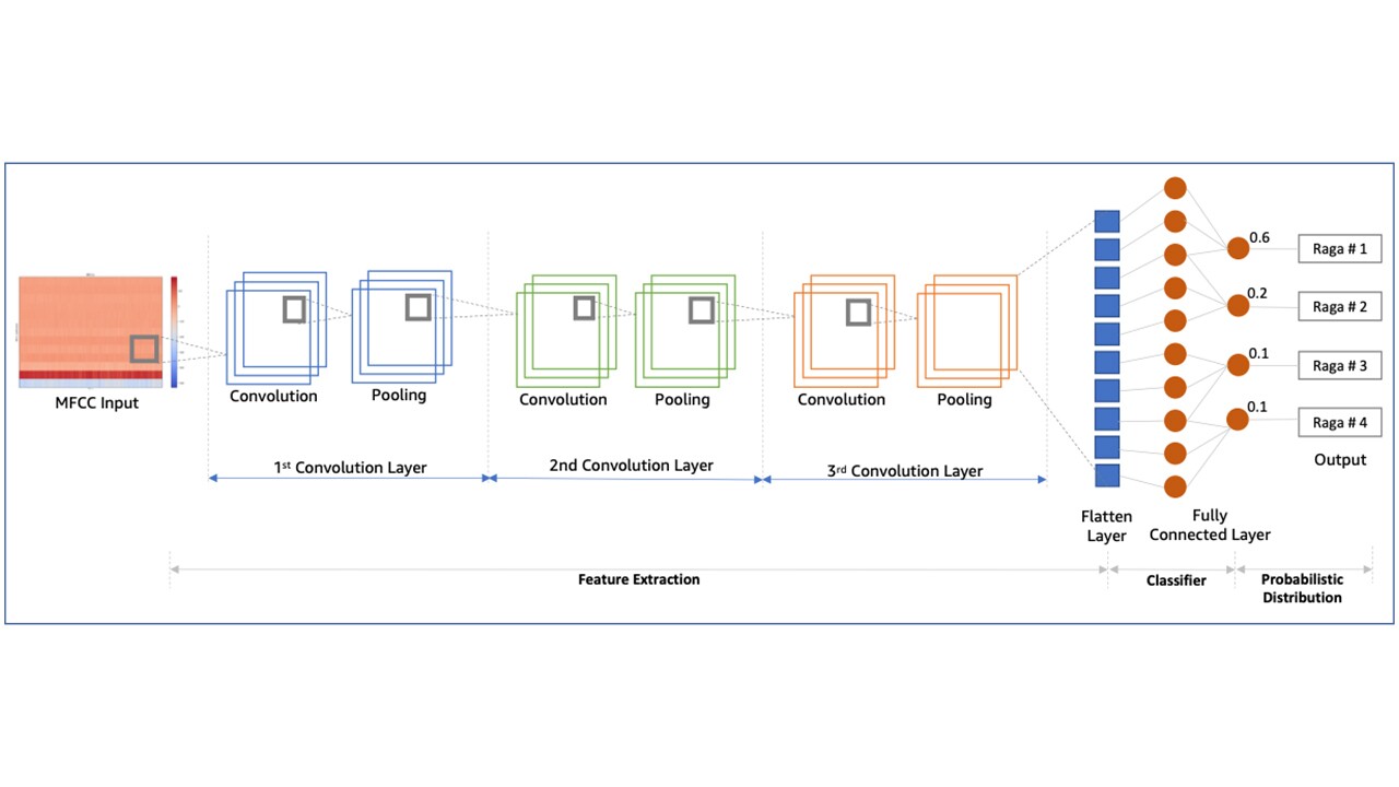
STEP 4 - INPUT DATA TRANSFORMATION : Convolutional Neural Network (CNN) was chosen to build the classifier. CNNs are not only effective for analyzing images, but also are effect for analysis of audio. This has been validated through multiple research findings. Please refer to the “References” section for such citations. However, what will be the input data shape fed to the CNN ? If we assume the hop length (refer to definition in the earlier sections) as 100, the total number of samples as 10,000, then we are talking about 100 (10000 / 100) such windows. The total number of MFCC is considered as 13, a typical number for music audio analysis. The input data shape is expressed as 100 x 13 x 1. The last dimension of “1”, is arguably redundant for this analysis. It is needed to match to the RGB (Red Green Blue) channel dimension, typical of an image input into a CNN. For audio segment represented through spectrogram and MFCC, it is set to 1 to match the data shape. This may be considered as a loose analogy to a grey-scale image data shape.

The diagram below outlines the CNN architecture that was used for this blog. The model was designed with three convolutional layers, using Adam optimizer, learning rate of 0.0001, relu as the activation function, and using softmax function to produce a probabilistic classification at the output layer.

The source code for this CNN was implemented using Keras. Keras is an open-source library build on Python for artificial neural networks. Keras is suitable for fast and simplified development, and more importantly it does support multiple backends such as Tensorflow. A developer can therefore switch to a different backend without significantly changing the front-ending Keras implementation layer. The section below outlines the code structure for model training.

# build network topology
model = keras.Sequential()

# 1st convolution layer
model.add(keras.layers.Conv2D(32, (3, 3), activation='relu', padding='same', input_shape=input_shape))
model.add(keras.layers.MaxPooling2D((3, 3), strides=(2, 2), padding='same'))
model.add(keras.layers.BatchNormalization())

# 2nd convolution layer
model.add(keras.layers.Conv2D(32, (3, 3), padding='same', activation='relu'))
model.add(keras.layers.MaxPooling2D((3, 3), strides=(2, 2), padding='same'))
model.add(keras.layers.BatchNormalization())

# 3rd convolution layer
model.add(keras.layers.Conv2D(32, (2, 2), padding='same', activation='relu'))
model.add(keras.layers.MaxPooling2D((2, 2), strides=(2, 2), padding='same'))
model.add(keras.layers.BatchNormalization())

# flatten output and feed it into dense layer
model.add(keras.layers.Flatten())
model.add(keras.layers.Dense(64, activation='relu'))
model.add(keras.layers.Dropout(0.3))

# output layer
model.add(keras.layers.Dense(10, activation='softmax'))

The model was compiled and trained with the following code:

# compile the CNN model
optimiser = keras.optimizers.Adam(learning_rate=0.0001)
model.compile(optimizer=optimiser, loss='sparse_categorical_crossentropy', metrics=['accuracy'])

history = model.fit(X_train, y_train, validation_data=(X_validation, y_validation), batch_size=32, epochs=75)

The model summary is printed as below:

model.summary()

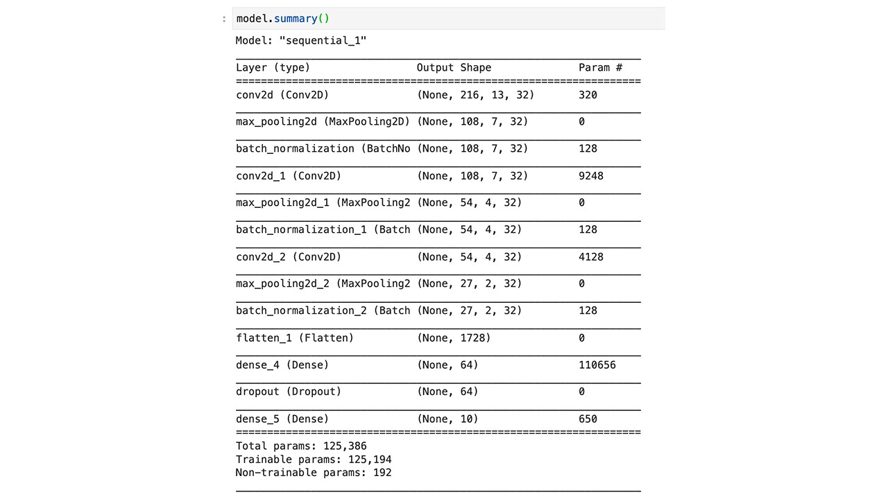
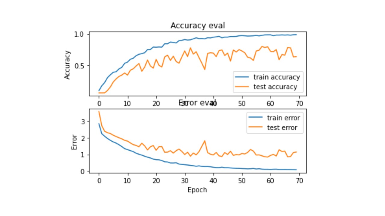
The image below is the model training history at a glance. It is important to validate that while a model has an increasing accuracy over the epochs, the test data (unseen to the model) also shows an improved accuracy and lowered error rates over the epochs of training. In TensorFlow, the history object does store the the accuracy and loss for both the train and test data across the epochs. The history object was used to plot this graph below. The model was trained for 75 epochs to obtain an initial accuracy of 72%, and with the first set of hyperparameters. An automated hyperparameter tuning exercise was conducted to further improve the model accuracy.

Machine learning models are refined and optimized through multiple iterations of training. The key input for each such iteration is a set of hyper-parameters that drive the training steps, and are kept constant during the training cycle. The potential combination of Hyperparameters for a deep learning model can grow exponentially, thereby making it difficult to run manual iterations and converge to the best of set of Hyperparameters for a given set of data, or training objective, or a use case. That is where automated Hyperparameter optimization techniques are useful to adopt. Amazon SageMaker provides a robust framework for such automated Hyperparameter tuning. This link provides a detailed overview of Amazon SageMaker Hyperparameter optimization.

The table below summarizes the first set of Hyperparameter while training the base model of CNN:

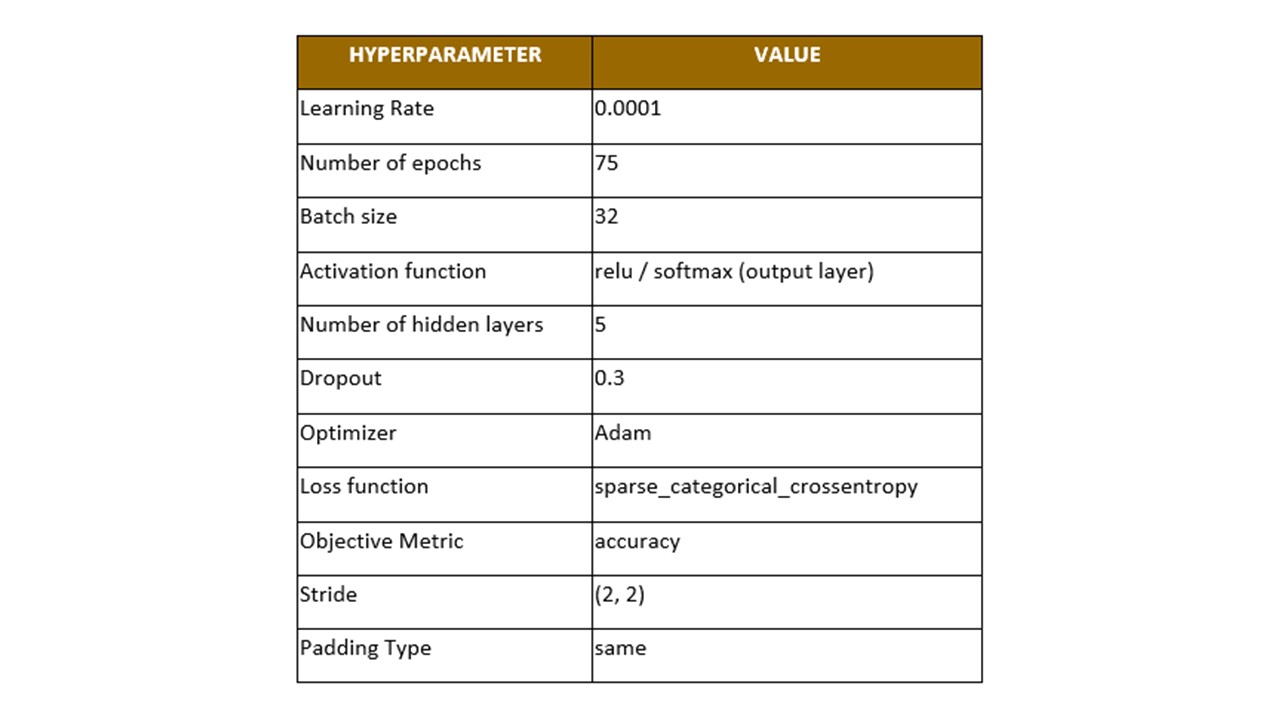
The base model accuracy was computed at 72% using the code snippet as below.

test_loss, test_acc = model.evaluate(X_test, y_test, verbose=2)

Hyperparameter tuning job was run on Amazon SageMaker. It did demonstrate significant improvement in the final objective metric, iterating through few cycles of Hyperparameter tuning. Please review the table below for reference.

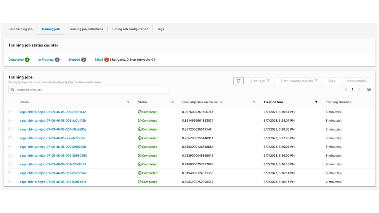
The best training job, associated with the best model with highest objective metric (92.7% , as outlined in the table above), was chosen for endpoint deployment. Please refer to this link for end-to-end instruction on how to setup a Hyperparameter tuning job on Amazon SageMaker.

Here are the key steps to be implemented to determine traces of Indian Raga within any song. These steps are guidelines and might need improvisation for specific use cases.

1. Obtain the target music file in a “wav” format. Most open source libraries for audio processing needs the input audio file in “wav” format.
2. Transpose the music pitch to match the pitch for which the ML model is trained. For example, if the model is trained for C# scale, the target audio pitch needs to be transposed as such. Music21 Python library, released by MIT under BSD license may be used as one of the tools for such pitch correction.
3. Depending on the target use case, considering separating out the vocals and instrumentals. A dominant percussion sound may suppress the melodic features of the song. This step is optional and depends on the type of music in consideration. Open sourced pre-trained classifier models may be explored to separate the vocals and instrumentals.
4. Split the song into segment size, same as what was considered for training the model (segments of five seconds). For each such segment, generate the MFCC and pass it as an input to the classifier model referred to above. Across the span of the song segments iteration, the positives and negatives are collected, to compute the average probability of a Raga presence.

It may be noted, that the computation approach to prediction can be simplified as tradeoff to how the CNN model is trained. For example, training with larger data set, ability to handle music in different pitches, or being trained on music with percussion instruments would imply higher time and costs for model training, but a more simplified and flexible inference mechanism.

This blog summarized a niche sub-domain of acoustically similar music classification, focusing particularly on Indian classical Raga system. The topics that were covered are - how selective audio features can be extracted, labelled, trained and tuned with machine learning. There is a substantial scope to develop further, by assembling larger data sets, reducing data bias & imbalance, experimenting with different CNN architectures, different audio features, etc. This concept can also be extended to world music, beyond the Indian Raga system. In western music dominant usage of major notes are known to emit a happy mood and dominant usage of minor notes emits a sad or tense emotion. Such note patterns can be analyzed, clustered and used for acoustically similar music classification. Once such “item-to-item” acoustically similar music items are clustered together, they can be used to power “you may also like” style of recommendations.

Last but not the least, this blog topic is at the intersection domain of technology, data science, and Indian classical music. For any product team to build a similar solution, the team has to be composed of such key skills such musicologists, data science and DevOps professionals.

The blog has been reviewed by Kapil Koul, who is a Software Development Director at Amazon specializing in security, privacy and governance for big data lakes that power analytics and machine learning use cases across Amazon.

1. Music Recommendation Based on Acoustic Features and User Access Patterns
2. Exploring Acoustic Similarity for Novel Music Recommendation
3. Emotional responses to Hindustani raga music: the role of musical structure
4. A hybrid social-acoustic recommendation system for popular music
5. Content-based Music Recommendation System
6. CNN Architectures for Large-Scale Audio Classification
7. Toward Universal Text-to-Music Retrieval -
8. Sample-level Deep Convolutional Neural Networks for Music Auto-tagging Using Raw Waveforms
9. India's rich musical heritage has a lot to offer to modern psychiatry
10. Study of Indian Classical Ragas Structure and its Influence on Human Body for Music Therapy
11. Immediate effect of listening to Indian Raga on attention and concentration in healthy college students
12. Emotional responses to Hindustani raga music: the role of musical structure
13. The sound of AI