Amazon, as a marketplace, is always thinking about how to match demand and supply, to create value for consumers and sellers. Building on vast stores of data available on the platform to do this, in Q1 2020, Amazon launched a product recommendation portal for seller partners on Amazon India that offers sellers insights consumer demand and preferences.
Every quarter Amazon comes up with a list of products which are in high demand by customers, but unavailable for purchase on Amazon.in because seller partners don’t offer them. We take this list of high demand products and match them with seller partners appropriately, based on their previously listed products on Amazon.in. We then display these matched recommendations on Amazon Seller Central to the respective seller partners so that they couldconsider listing these products to sell on Amazon.in.
The matching and recommendation of products are unique and tailored to individual seller partners, based on only their data. A seller partner can only see their own recommendations; by default, the product recommendation portal shows recommendations to the seller partner on the basis of their primary selling category as seen below.
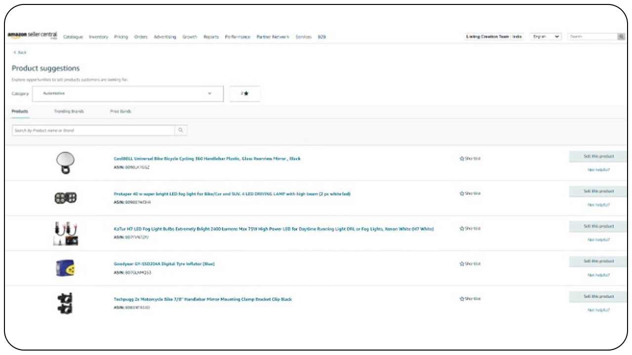 A screengrab of the Product Recommendation Portal that a seller can see.
In case the seller partner is interested to view recommendations in other product categories then they can choose a different category from the category dropdown menu.
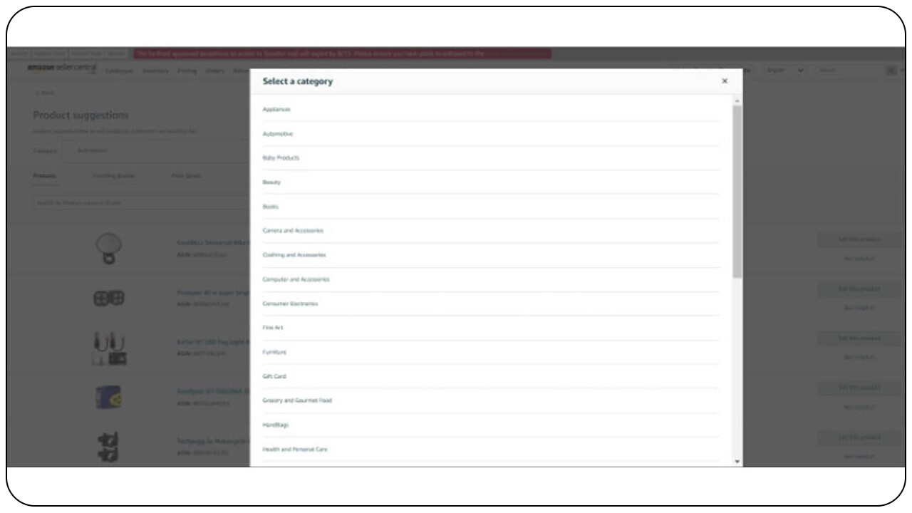 A screengrab of how to view recommendations from different product categories.
We then refresh the recommendations that are matched to them for the newly selected category.
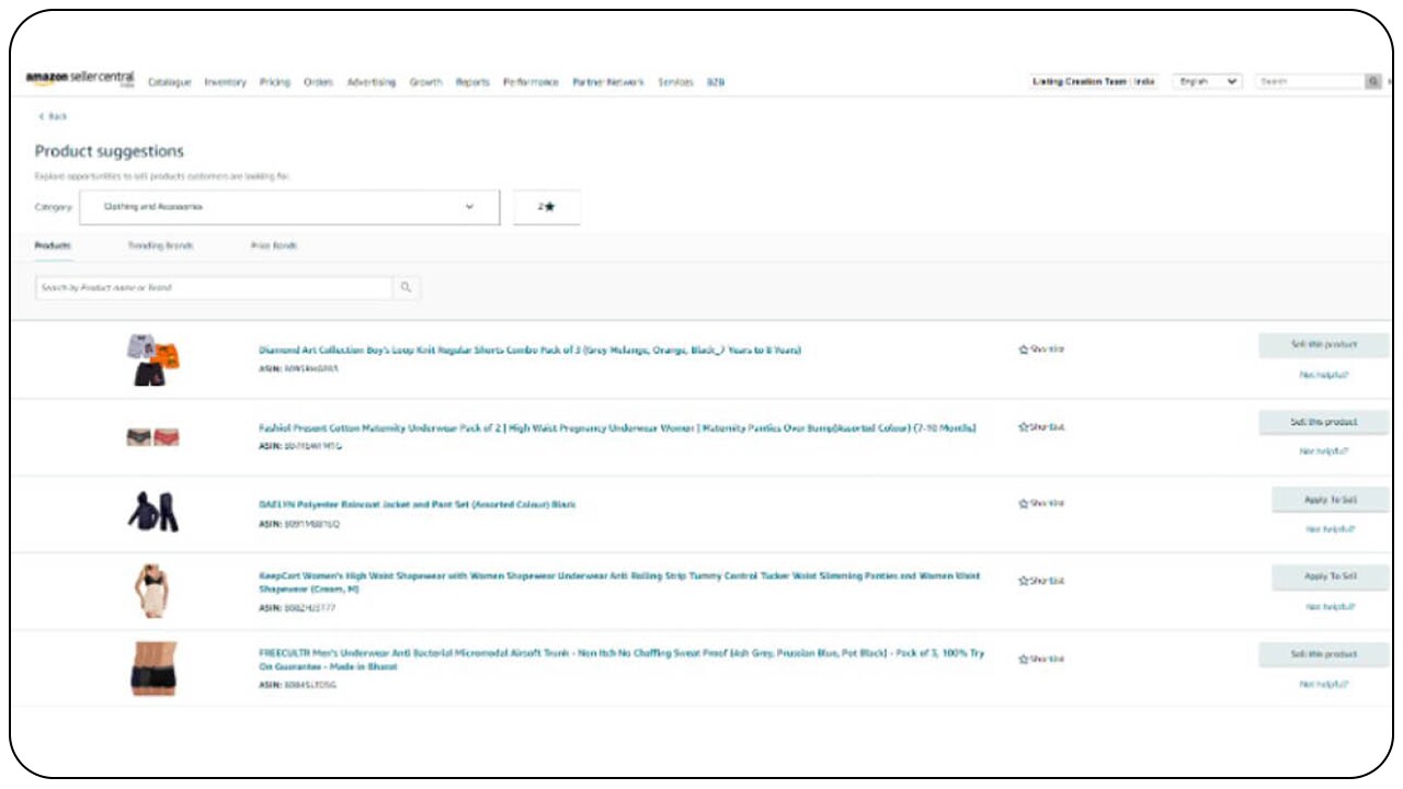 A screengrab of refreshed recommendations basis a seller's choice.
This article describes the basics of how we built the recommendation system, and dives deep into the challenges faced and how we solved them.
Fundamentals of how we built our recommendation system
Our recommendation system is based on User-Item Collaborative Filtering (CF) paradigm. In our case, the users of our recommendation system are seller partners and items are products sold on Amazon.in. When seller partners (SP) have already offered a particular product (P) we consider that <SP, Product> pair as a positive pair, and any pair where SP hasn’t offered the product is considered a missing pair. We represent this data as a matrix (affinity matrix) with each row representing a SP and each column representing a product. If SP has listed the product on Amazon.in, the corresponding cell has a value of 1 and if SP hasn’t listed the product, the corresponding cell is empty.
In the example below, for a group of 4 seller partners (SP) and 6 products (P), the matrix can be read as:
- S1 has listed product P1, P4, P5 for selling on Amazon.in
- S2 has listed P2, P4, P5
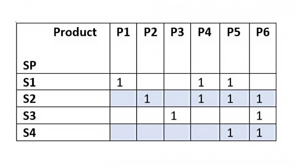
To recommend new products to seller partners we need to complete the above matrix, which would tell us about seller partner’s affinity to list a product they haven’t already listed. To complete the matrix, we fill the empty cells with a score between 0 to 1, with 0 indicating that the product is unsuitable to be recommended while 1 indicating perfect suitability for recommendation. We set threshold as 0.5, below which we consider the score to be unsuitable for recommending the respective product to the seller partner.
For example, a possible completion for the above matrix can be as below :
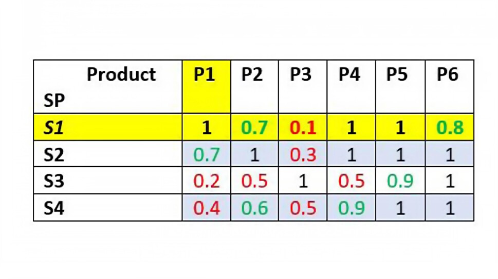
Using the completed matrix above, we can now see that for S1, P2 and P6 are good recommendations, but P3 isn’t a good recommendation. There are multiple algorithms to obtain the matrix completion which include matrix factorization and link prediction using graph neural networks.
Sparsity challenges with matrix completion method
While the example in the above section had only 4 seller partners and 6 products, in our use case we cater to all seller partners on Amazon.in which is over 300K and our high demand product list is over 100K products. Conversely most seller partners list fewer than 100 products for selling on Amazon.in. As a consequence, the affinity matrix is very sparse with few cells filled and most cells in the matrix remaining empty.
We can define sparsity as :
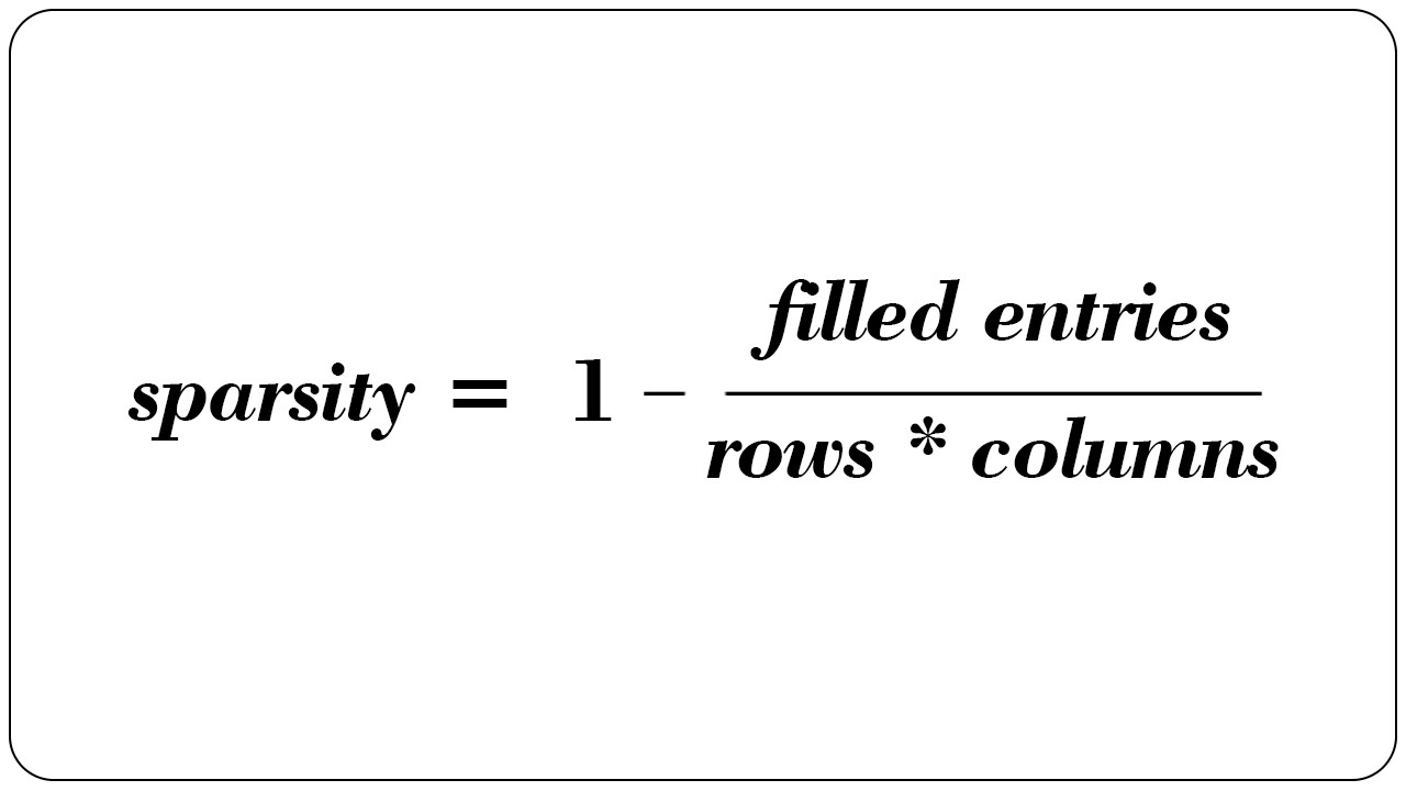
In our example the sparsity is 1 - 11 / (4*6) = 0.55; in other words, 45% of the cells in affinity matrix are already filled from available data and 55% cells are empty. For our actual use case the sparsity was over 0.9999 or only 0.01% of the cells in the affinity are filled from available data and 99.99% cells are empty. Matrix completion methods depend on filled cells of affinity matrix to infer the empty cells, using each filled cell as a training example. As a consequence, when the proportion of filled cells is higher these methods provide a better estimate of the empty cells and vice versa. High sparsity leads to low accuracy of the recommendation algorithm. We discuss the steps we took to alleviate sparsity and produce optimized recommendations for all seller partners in the next sections.
Adapting graphs and link prediction to solve sparsity problem
To address the sparsity problem by using more data sources present at Amazon.in, we adopted the link prediction using graph neural networks method to estimate the empty cell values of the SP, Product affinity matrix.
For an overview of graph neural network and training look at A Gentle Introduction to Graph Neural Networks, Understanding Convolutions on Graphs, DGL introduction and Link prediction with DGL.
In this method, we use a graph of our data and convert each seller partner and product into a node in the graph. For our example seller partners S1 to S4 are shown in red and Products P1 to P6 are shown in blue. Edges (or links) between these nodes represent whether seller partner listed a particular product. The problem of matrix completion can now be solved as link affinity prediction where we try to predict the affinity score for the missing links in the graph between Seller Partners and Products
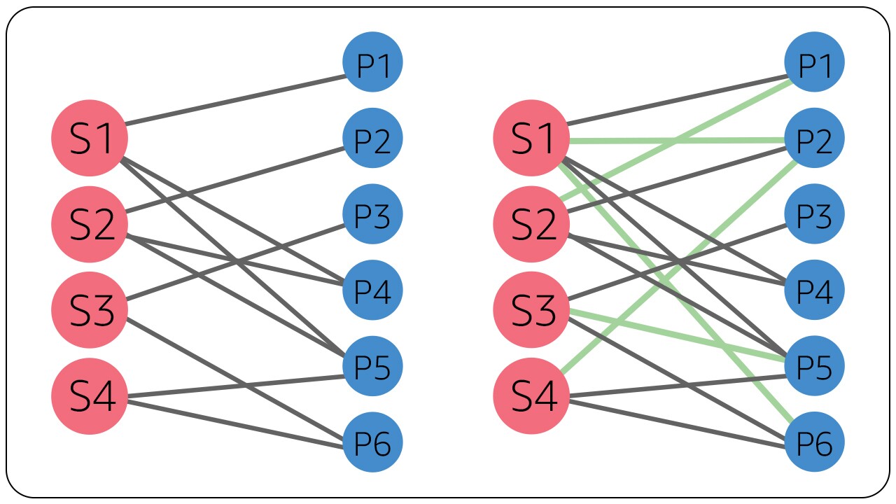
In the figure above in left we see how the graph appears without links being completed, while on right we show the completed links using link prediction in green. Notice that in this solution also P2 and P6 are the best suggestion for S1.
Here, adapting the graph structure provided us with the capability to utilize other relational data sources. We augmented the graph with additional products and new edges.
- We augmented our graph with additional products which have a high number of clicks on Amazon.in; these additional products will not be recommended to seller partners but their presence will help in the training of our link prediction model. We added over 2 million such products to the graph.
- We also added new edges to the graph by looking at products which were bought together by the same customer (“customers who bought this also bought”). For example, a mobile phone and its corresponding cover case are bought by the same customer, and as such, these edges can tell us the relationships between products. To ensure that we only sample relevant edges, we only consider product pairs bought by the same customer within 7 days. We also apply a count threshold and take only those product pairs which have higher occurrence over our count threshold in a 7-day window.
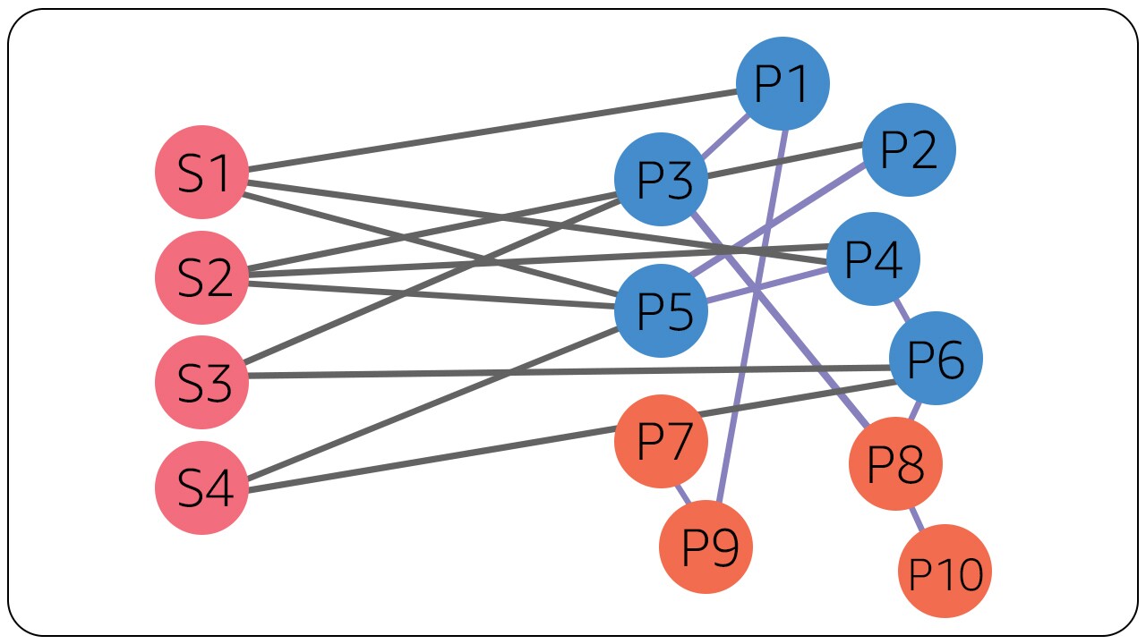
With these two changes our graph would appear as below. You can notice that here we added 4 additional product nodes in orange with links between product nodes (in blue) using customer purchases. This reduces graph sparsity for high demand product nodes (P1 to P6), providing more edges per product node and enables us to train our link prediction model better.
Results of augmented the graph with additional products and new edges
- The addition of about 2 million additional products as nodes to our graph resulted in increasing our model training time. The training time is proportional to the number of nodes + edges, training time ∝ O(V+E) and hence our training time increased by over 10x.
- Additionally, the newly added product nodes have higher connectivity (edge per node) compared to the high demand product nodes that we want to recommend to our seller partners. Due to this, the high demand product nodes are seen less frequently by the model during training since we used simple random graph edge sampling for training our model. The model would be less capable of providing accurate affinity scores between seller partners and high demand product nodes, while the training loss and affinity scores for additional nodes, edges will be good.
Using product features and graph edge sampling to solve scaling challenges
In order to scale our model, we proposed to reduce dependence on graph training and incorporate product features such as title and product attributes. Product title and attributes are available on the product detail page as shown below.

We convert these details into a vectorized format using an NLP text to vector model like BERT and Doc2Vec. We thus obtain a n-dimensional vector (Pvec) for each product, for creating vectors for seller partners (Svec) we take weighted average of vectors of their listed products. The vector weights are determined by how many product page views each product offered by the seller partner received in the last N months.
For example S1 has listed products P1, P4, P5, and let their product page views be v1, v4, v5, then S1’s vector representation is computed as below.
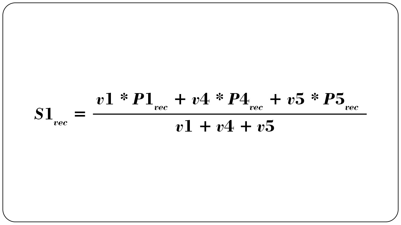
These vector representations computed from product attributes/features are closer in the vector space if the products are similar. An iPhone 12 and iPhone 12 case cover would be closer than iPhone 12 and Samsung Galaxy S20 case cover due to their product titles. Hence using these representations S1vec will be closer to P1vec, P4vec, P5vec and to any other product vectors which are closer to P1vec, P4vec or P5vec. We can then use a K-nearest neighbor retrieval algorithm to retrieve products closest to seller partner S1.
While product attribute-based vector representations reduce compute time, this method doesn’t utilize additional node, edges obtained by product pairs purchased by same customer. To ensure that additional nodes and edges are utilized we further train these vectors using link prediction model that was built earlier. Product attribute-based vectors are used to initialize the link prediction model instead of random initialization.
To prevent over-representation of additional product nodes in training samples and provide accurate affinity scores between seller partners and high demand product nodes while reducing our training duration, we adopted stratified edge sampling with the below rules.
- Sample only <seller partner, product> edges as root nodes for graph neural network.
- For each seller partner sample only edges where the product is a high demand product or belongs to top-3 viewed product (on basis of product page view on amazon.in) among all the products the seller partner has listed.
- At any non-root layer sample only 3 edges for a node.
- Truncate depth of graph neural network at 4 layers.
Rule 1 and 2 reduce the number of nodes and edges sampled for training, while Rule 3 and 4 reduce neural network compute for each training example. With these changes we are able to reduce training time despite addition of extra nodes and edges.
Results
In the above sections we made several changes to our initial model to obtain better model performance and improve product recommendations to our seller partners while optimizing compute for graph neural network training. Here we present our results by comparing it with a Matrix Factorization baseline. We look at Recall@100 which is defined by taking the top 100 recommendations made by our model for a seller partner and comparing it with seller partners actual listed products. We then average the Recall@100 for all seller partners to compute our final metric reported in table below.
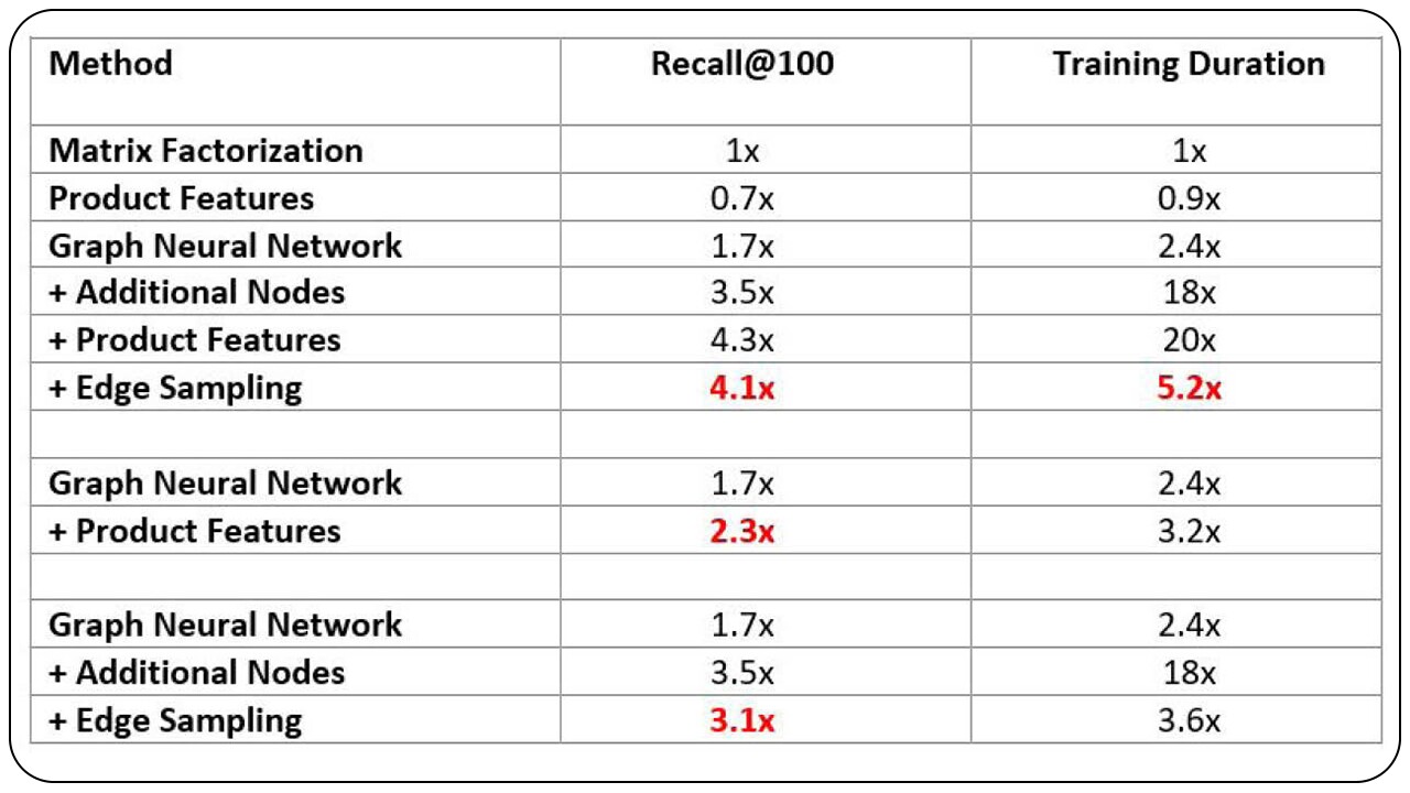
As we can see from the table above, adding product features and additional product nodes enhances Recall@100 metric of our network, while also increasing the compute required by ~20 times. To compensate for this, our edge sampling strategy reduces the number of nodes, edges used for training as well reduces the per-step compute of the network. All these changes together provide a 4x increase in Recall@100 while optimizing compute without compromising much on the accuracy.
Final thoughts
While building machine learning systems many careful choices on both data and algorithm have to be made. Key learnings on making such choices that we can take from this work are:
- Take a close look at data sparsity: In many machine learning problems, presence of data sparsity causes common algorithms to yield suboptimal performance. In our case, matrix factorization did not perform optimally due to sparsity in affinity matrix of our recommendation system.
- Find sources of relational data to alleviate sparsity: Relational data is present in a variety of forms in various scenarios. In e-commerce platforms, customer-product, seller-product, product-product relationships can be derived. Similarly in other platforms like social networks, we can derive relationships by using user-post interactions and user-user interactions. In general, taking a look at the various entities involved and their interactions provides an idea of what relations between entities can be derived. Relational connections allow us to represent one entity using not only its own data but also data from other entities, thereby reducing the impact of data sparsity.
- Use Graph Neural Networks to incorporate relational data: A key deep learning architecture to handle relational data is Graph Neural Network (GNN). Traditional methods were designed to handle data of the current entity in a training sample, but GNN is designed to handle data of the current entity as well as connected entities for training the model. Use of additional relational data in the model alleviates data sparsity issues and provides better performance compared to traditional algorithms.
- Perform data sampling on the basis of use case: Addition of relational data increases compute requirements. To reduce compute demand various sampling techniques can be used. GNN models allow customizing graph depth as well as expansion factor per level which can be tuned to achieve right compute-performance trade-off. Sampling on the basis of use case can lead to further improvements, e.g., main entity in our use case were our seller partners, hence we sampled root edges for GNN which had seller partner as a node, while we used other edges like product-product edges for later GNN layers.